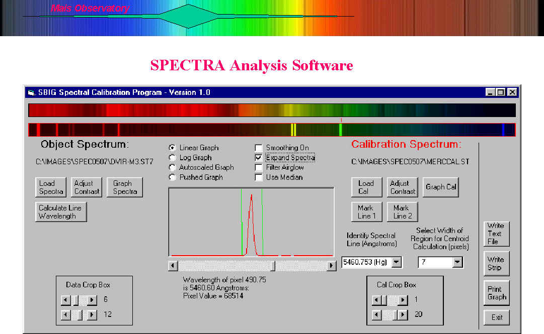
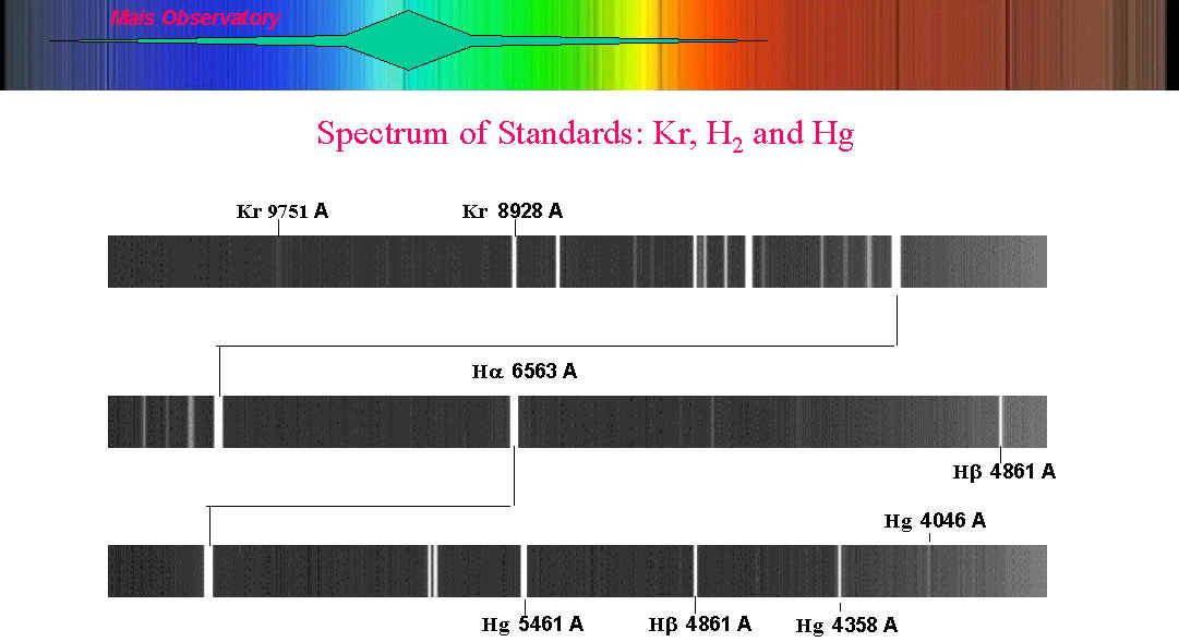
There are two parts to calibration following the usual dark subtraction flat fielding and this consists of wavelength 

and flux calibration. The Self guided Spectrometer comes with software called Spectra which allows you to 

calibrate the wavelength using, ideally, gas emission tubes which emit distinct lines at known wavelengths. 

I use hydrogen and mercury lamps which are fed by fiber optics to a window on the bottom of the spectrometer. 

This allows me to imprint my spectra with known emission lines. For wavelengths greater than 7000 angstroms, 

I also use a krypton emission tube.

                        SPECTRA software window                                             Emission spectra of Kr, Hg and H₂

__________________________________________________________________________________________________

For flux calibration, one first obtains data from standard stars such as 108 Virginis. Graphically, the spectrum of

108 Virginis is shown below in Figure 1. One can also download data from a Spectrophotometric Database Site into a spread 

sheet such as Excel, a small

                                                                                                  Figure 1

__________________________________________________________________________________________________

spectral slice is shown in Figure 2. Using this data, one converts the magnitude of the standard for a wavelength 

interval(16 angstroms) into a number of photons/cm²/sec/nm using the formula F_l = 5.5x10(1/l)10^-0.4mag. 

Next one obtains a spectrum, in this case 108 Virginis through the optical train of your set up. The top graph 

in Figure 3 shows the spectrum obtained with my system. By using SPECTRUM software for wavelength

__________________________________________________________________________________________________

                                                                                                                         Figure 2

____________________________________________________________________________________________________________________

calibration, one can save the wavelength calibrated file as a text file and import into Excel. This gives you wavelength in one 

column and raw counts in the other column, a small portion of which is seen in the first two columns showed in bottom table of 

Figure 2. Raw counts/pixel can be converted to photons/pixel based on the gain of your camera and finally photons/cm²/sec/nm 

depending upon your telescope aperture and wavelength range (columns 3 and 4 in bottom table of Figure 2). Finally, dividing 

your number into that for the standard star (column 5, bottom table of Figure 2) you obtain a correction factor which can be 

applied to your text data. In Figure 3, the top graph is the un-calibrated graph while the bottom one represents the graph 

following application of the correction factor across spectrum. See Sky and Telescope, July 2000 page 125-132 for further 

details on this procedure. 

________________________________________________________________________________________________________

                                                                                     Figure 3

________________________________________________________________________________________________________________

Figure 4 allows you to see directly the comparison of the spectra between 108 Virginis from the spectrophotometric 

database and the flux corrected graph as obtained through my particular setup. For more exacting work, one would 

have to allow for atmospheric extinction, but this gives a good first order calibration. The correction factors obtained 

can be used over and over again for other spectra.

________________________________________________________________________________________________________________

                                                                                                                                Figure 4